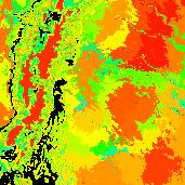
SOM Eto (Variable) Classification
Yachay Tech's SomEto project proposes the use of the artificial intelligence method called Self Organizing Maps (SOM) to classify standard evaporation (ETo) areas based on the WRF variables used to calculate ETo. Note that the SOM does not actually calculate ETo but instead uses ETo input variables to classify. In the examples below, only raw variable values are used, eg. water ratio instead of relative humidity, wind components instead of magnitude, etc.
A "shallow" learning was implemented for the Andean region of Ecuador, by taking only one time slice, at 12:00pm every day, over the month of May, 2020. The animation below shows subsequent classification of the region over the period 2020-06-01 to 2020-10-14, based on the learning from May. There are 64 classes over 171x171 pixels, at 3km pixel resolution. The data used was not normalized.
Ecuador 64 Classes 06/01 to 10/14
The animation below shows the same region and time but with normalized data and 16 classes.
Ecuador 16 Classes 06/01 to 10/14
Our preliminary research involves determining appropriate data preparation. Do we use raw or refined values (eg. water ratio -> relative humidity)?. Should the variables be weighted, normalized, or normalized and weighted? What is our measure of success?
Our measure of success is to achieve a stable classification of areas with minimal migration. The top animation shows a fairly stable mountainous classification, while the Amazonia and western regions are more volatile. This could be due to the non-normalized presentation, skewing the classification to higher valued variables such as temperature. However, it is worth mentioning that Demartines and Bayo (1992) showed that high dimensional (about 12 or more) SOM implementation does not require normalization. We are using 10 dimensions in our feature space.
The bottom classification animation uses normalized data, but mountainous area stability only occured when using smaller network geometry. Note that in our implemention we are asking the SOM to replicate the difference in areas that would normally be differentiated by calculating ETo, which is distinct from most AI applications clustering where there is no equation, only parameters in the feature space (variables). We intend to address data preparation through sensitivity studies involving normalization and weighting of the variable as they would contribute to the ETo equation.
The animations below show the same region using a "deeper" learning by incorporating hourly values over the months of March, April, and May.
Ecuador 64 Classes 06/01 to 10/14
Ecuador 36 Classes 06/01 to 10/14
The above SOM classification animations used WRF raw variables, specifically, TSK, EMISS, SWDOWN, GLW, GRDFLX, T2, PSFC, Q2, U10, V10. From these we derive the necessary variables for the Penman-Montieth equation: Rn, G, Thc, D, g, es, ea, w2. The animation below shows classifications usng these derived variables. Training used hourly values over the months March, April, and May.
Ecuador 64 Classes 06/01 to 10/14
The animation below shows the classification using normalized values of the derived variables.
Ecuador 64 Normalized Classes 06/01 to 10/14
It is evident that deeper learning is accomplished with larger data set presentation. The above exercise shows how the transition from one time slice to twenty-four slices helps differentiate very subtle aspects of evaporation and converges toward a more stable (less migration) classification over time (see Amazonia region in first and third animations above).
Understanding that migration of ETo classifications over time is inevitable, due to environmental shifts, our task is to first achieve classifications with minimal migration. This then allows for a general and flexible categorization of ETo environments. For example, if pixel A only takes on u, v, w classes throughout a year then it and other pixels which only take on u, v, w classes would share a common ETo environment, or category.
To characterize the migration behavior of classes on a pixel over a time period and then identifying "similar" pixels can be daunting, with over 2.6 million samples for a 3 month run. Here we turn to SOM once again to interpret similar pixels, or to cluster, based on classifications over time. The image below shows a clustering of the derived ETo classification over time period 2020-0601 to 2020-10-14

Our goal is to pursue the above issues and to implement a "deeper" learning method by incorporating hourly time slices, over years and over larger regions, into the data presentation for SOM weather classification research.